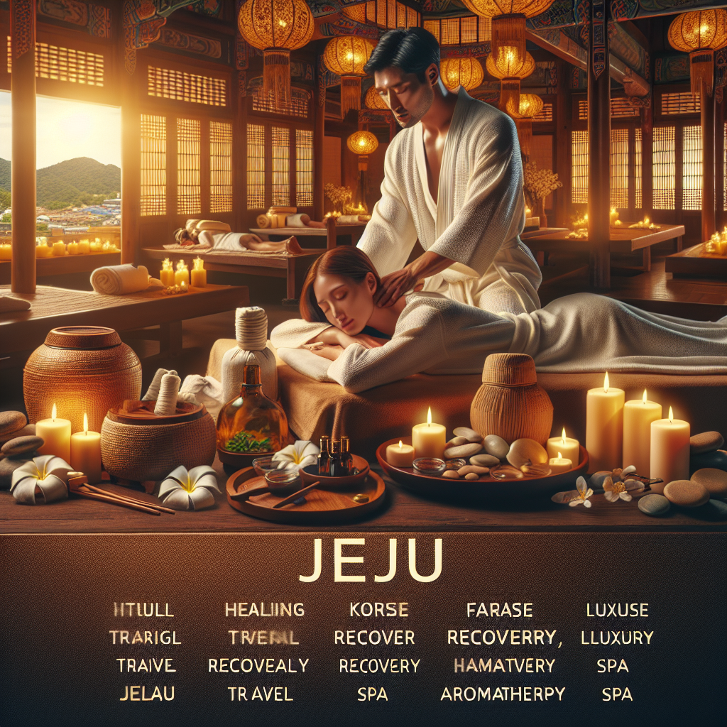
제주 힐링 마사지 추천: 자연과 힐링이 만나는 공간
안녕하세요, 여러분! 제주도는 아름다운 자연과 푸른 바다로 유명한 힐링의 섬이죠. 이곳에서의 휴식은 단순한 여행에서 벗어나 진정한 힐링을 경험할 수 있게 해줍니다. 그중에서도 제주 마사지, 특히 힐링 마사지는 몸과 마음을 편안하게 만들어주는 필수 코스입니다. 오늘은 제주에서 꼭 경험해봐야 할 마사지 추천과 그 효능에 대해 이야기해보려고 합니다. 제주는 뛰어난 자연 환경 속에서 다양한 스파와 마사지샵들이 운영되고 있어,…

브랜드 스토리텔링 전략: 성장을 위한 길잡이
현대 사회에서 소비자는 단순한 제품이나 서비스 이상의 가치를 원합니다. 그들은 브랜드에 대한 연결과 감정을 중시하며, 이러한 요구를 충족시키기 위해 ‘브랜드 스토리텔링’이 필요합니다. 브랜드 스토리텔링이란 소비자와의 관계를 깊게 만들기 위한 이야기 전달 방식입니다. 이 전략은 브랜드가 어떻게 성장할 수 있는지를 명확하게 보여줍니다. 브랜드의 성장은 단순히 매출 증대나 시장 점유율 확대만을 의미하지 않습니다. 진정한 성장은 고객과의 관계…
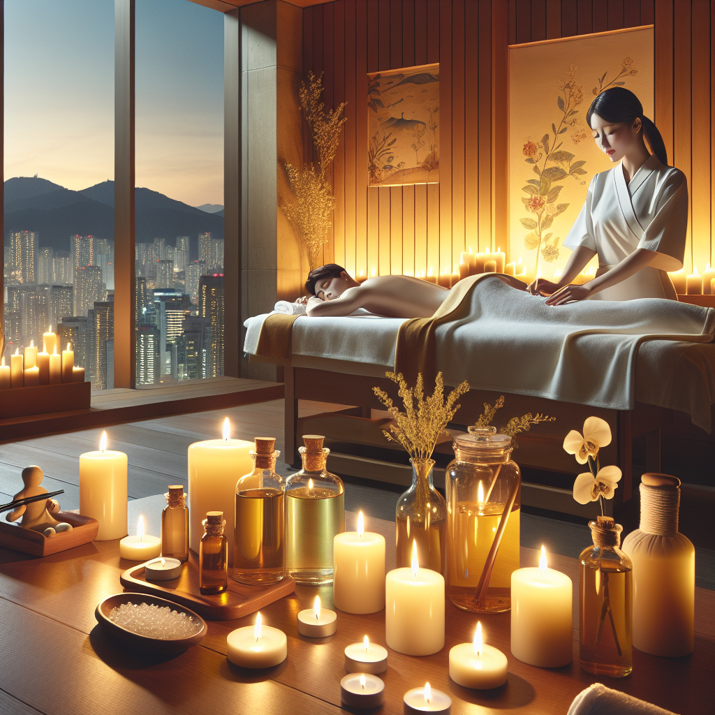
커플을 위한 제주 럭셔리 마사지
제주도는 아름다운 자연경관과 함께 평화로운 분위기로 유명합니다. 이곳은 사랑하는 사람과의 특별한 시간을 보내기에 최적의 장소인데요. 특히 커플들이 함께 즐길 수 있는 제주 마사지는 더욱 특별한 경험을 선사합니다. 제주 럭셔리 마사지는 단순한 휴식을 넘어서 커플의 서로에 대한 이해와 애정을 더 깊게 해주는 시간이 될 수 있습니다. 이곳의 고급 스파와 마사지 서비스는 모두가 편안함을 느낄 수 있도록…
휴식과 여유를 주는 부산 스파 체험
바쁜 일상 속에서 피로감을 느끼는 순간, 우리는 종종 휴식이 필요하다는 것을 실감합니다. 그러한 가운데, 부산은 아름다운 해안선과 더불어 다양한 스파 시설로 유명합니다. 이 글에서는 부산 스파를 통한 편안한 휴식과 여유를 경험할 수 있는 방법을 소개하고자 합니다. 부산 스파는 그동안 사람들에게 인기를 끌어온 휴식 공간입니다. 도시의 분주함을 잊고, 자연과 조화를 이루며 힐링하는 공간으로서 많은 이들에게 사랑받고…
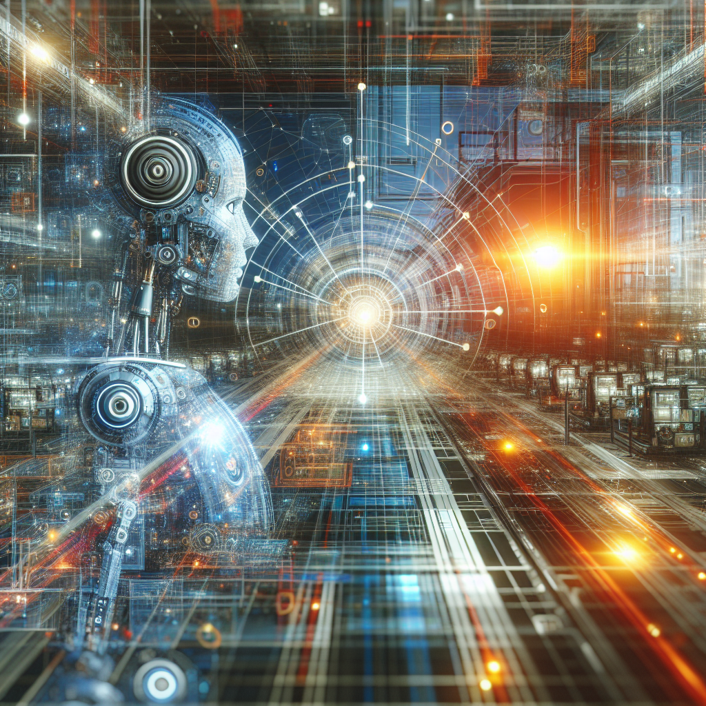
AI가 바꾸는 미래 산업 구조
AI가 바꾸는 미래 산업 구조 우리는 기술이 발전함에 따라 사라지거나 변모하는 직업들을 목격해 왔습니다. 특히 인공지능(AI)의 등장은 우리 삶의 많은 부분을 변화시키고 있으며, 이는 산업 구조에 상당한 영향을 미치고 있습니다. AI는 비즈니스 모델을 혁신하고, 새로운 기술적 가능성을 열어줍니다. 하지만 이러한 변화는 단순히 기술의 발전으로 끝나는 것이 아니라, 우리의 일하는 방식과 사고 방식을 재정의하고 있습니다. AI…

오늘의 뉴스: 최신 트렌드가 가져오는 변화
안녕하세요, 오늘도 따뜻한 소식으로 돌아온 블로그입니다. 우리는 매일 새로운 뉴스와 정보를 접하고 있죠. 오늘은 그중에서도 특별히 최신 트렌드에 대해 이야기해보려 합니다. 세상은 빠르게 변화하고 있으며, 그 변화 속에서 우리는 어떤 것들을 살펴볼 수 있을까요? 오늘의뉴스 우리가 살고 있는 이 시대에는 변화가 일상이 되었습니다. 특히 기술의 발전과 함께 최신 트렌드가 그 중요성을 더해가고 있습니다. 기업에서 개인…
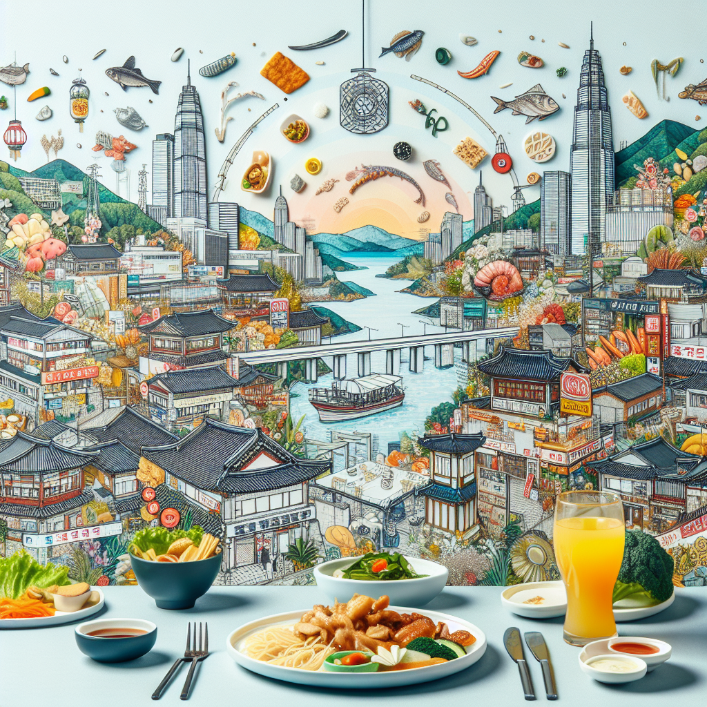
부산 맛집 추천: 맛과 분위기를 모두 갖춘 곳들
부산 맛집 추천: 맛과 분위기를 모두 갖춘 곳들 부산, 우리나라 제2의 도시로서 아름다운 해안선과 더불어 다양한 음식을 자랑하는 곳입니다. 여행객뿐만 아니라 현지 주민들까지 즐겨 찾는 부산 맛집을 소개해드리려고 합니다. 맛있는 식사와 멋진 풍경이 어우러지는 경험을 통해 부산을 더욱 가깝게 느껴보세요. 1. 해운대의 시원한 바다를 보며 즐기는 회 해운대는 부산의 대표적인 해수욕장으로, 바다를 바라보며 회를 즐길…
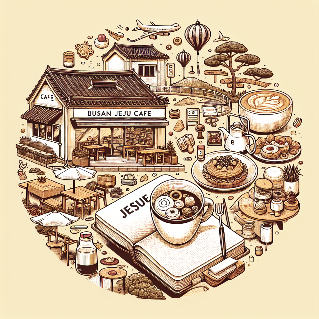
제주카페에서의 특별한 하루
제주카페에서의 특별한 하루 안녕하세요! 오늘은 따뜻한 제주에서 만날 수 있는 특별한 카페들을 소개해 드리려고 합니다. 제주카페는 단순히 커피와 디저트를 즐기는 곳 이상의 의미를 가집니다. 각각의 카페는 그들만의 독특한 분위기와 매력을 가지고 있으며, 제주도의 아름다운 자연과 완벽하게 어우러져 그 자체로 하나의 여행지가 되기도 합니다. 제주카페의 매력 제주카페는 바다의 푸른 물결과 하늘의 맑은 색이 조화를 이루는 곳에…
AI로 돈 버는 방법: AI부업으로 새로운 수익 창출하기
AI로 돈 버는 방법: AI부업으로 새로운 수익 창출하기 요즘 들어 인공지능(AI)이 점점 더 많은 사람들의 일상에 스며들고 있는 것을 감지할 수 있습니다. 우리가 매일 사용하는 스마트폰, 가전제품, 심지어 인터넷 포털 사이트까지도 AI의 혜택을 보고 있습니다. 이러한 변화는 수많은 기회를 우리에게 제공합니다. 특히 ‘AI부업’을 통해 새로운 수익을 창출하는 방법에 대해 이야기해보려 합니다. AI부업이란 무엇인가? AI부업은 인공지능…